小白劝退预告

仅简单介绍思路，没有用作教程的打算，如果读者没有深度学习基础、计算机视觉基础、Pytorch基础 —— 会很不友好的(

前置准备

我们先准备好对应的第三方模块包和使用函数

import torch
from torch import nn, optim
import torch.nn.functional as F
from torchvision import datasets, transforms
from torch.utils.data import DataLoader
import matplotlib.pyplot as plt
from time import perf_counter

我们先写好一个展示神经网络结构并输出张量形状的函数
showModel 通过递归调用，将所有 Sequential 类展开，并以此输出各层的张量大小
showNet 通过输入模型，并指定张量的大小，实现了测试函数的封装

def showModel(model, inputs):
    for layer in model:
        if layer.__class__.__name__ == "Sequential":
            inputs = showModel(layer, inputs)
        else:
            inputs = layer(inputs)
            print(f"%20s output shape : {inputs.shape}"%(layer.__class__.__name__))
    return inputs

def showNet(model, input_size):
    inputs = torch.randn(input_size)
    inputs = showModel(model, inputs)
    print(inputs)
    return

我们先创建一个神经网络，并测试上述函数的作用
我们发现这个函数实现了我们需要的功能

showNet(
    nn.Sequential(
        nn.Sequential(
                    nn.Conv2d(1, 96, kernel_size=11, stride=4), nn.ReLU(),
                    nn.MaxPool2d(kernel_size=3, stride=2),
                    nn.Conv2d(96, 256, kernel_size=5, stride=1, padding=2), nn.ReLU(),
                    nn.MaxPool2d(kernel_size=3, stride=2),
                    nn.Conv2d(256, 384, kernel_size=3, stride=1, padding=1), nn.ReLU(),
                    nn.Conv2d(384, 384, kernel_size=3, stride=1, padding=1), nn.ReLU(),
                    nn.Conv2d(384, 256, kernel_size=3, stride=1, padding=1), nn.ReLU(),
                    nn.MaxPool2d(kernel_size=3, stride=2),
            ),
            nn.Sequential(
                    nn.Flatten(),
                    nn.Linear(256 * 5 * 5, 4096), nn.ReLU(),
                    nn.Dropout1d(p=0.5),
                    nn.Linear(4096, 4096), nn.ReLU(),
                    nn.Dropout1d(p=0.5),
                    nn.Linear(4096, 10),
                    nn.Softmax(dim=1),
            )
    ), 
    (1, 1, 224, 224),
)

Conv2d output shape : torch.Size([1, 96, 54, 54])
ReLU output shape : torch.Size([1, 96, 54, 54])
MaxPool2d output shape : torch.Size([1, 96, 26, 26])
Conv2d output shape : torch.Size([1, 256, 26, 26])
ReLU output shape : torch.Size([1, 256, 26, 26])
MaxPool2d output shape : torch.Size([1, 256, 12, 12])
Conv2d output shape : torch.Size([1, 384, 12, 12])
ReLU output shape : torch.Size([1, 384, 12, 12])
Conv2d output shape : torch.Size([1, 384, 12, 12])
ReLU output shape : torch.Size([1, 384, 12, 12])
Conv2d output shape : torch.Size([1, 256, 12, 12])
ReLU output shape : torch.Size([1, 256, 12, 12])
MaxPool2d output shape : torch.Size([1, 256, 5, 5])
Flatten output shape : torch.Size([1, 6400])
Linear output shape : torch.Size([1, 4096])
ReLU output shape : torch.Size([1, 4096])
Dropout1d output shape : torch.Size([1, 4096])
Linear output shape : torch.Size([1, 4096])
ReLU output shape : torch.Size([1, 4096])
Dropout1d output shape : torch.Size([1, 4096])
Linear output shape : torch.Size([1, 10])
Softmax output shape : torch.Size([1, 10])
tensor([[0.1006, 0.0992, 0.1000, 0.0991, 0.1017, 0.0995, 0.1013, 0.0994, 0.1002, 0.0991]], grad_fn=)

LeNet

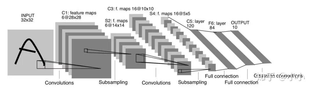
Lenet 是一系列网络的合称，包括 Lenet1 - Lenet5，由 Yann LeCun 等人在 1990 年《Handwritten Digit Recognition with a Back-Propagation Network》中提出，是卷积神经网络的 HelloWorld

Lenet是一个 7 层的神经网络，包含 3 个卷积层，2 个池化层，1 个全连接层。其中所有卷积层的所有卷积核都为 5x5，步长 strid=1，池化方法都为全局 pooling，激活函数为 Sigmoid，网络结构如下：

LeNet的网络架构

# input_size  (1, 1, 32, 32)
# output_size (1, 10)
class LeNet(nn.Module):
    def __init__(self):
        super(LeNet, self).__init__()
        self.conv = nn.Sequential(
            nn.Conv2d(1, 6, kernel_size=5, stride=1),
            nn.MaxPool2d(kernel_size=2),
            nn.Conv2d(6, 16, kernel_size=5, stride=1),
            nn.MaxPool2d(kernel_size=2),
        )
        self.linear = nn.Sequential(
            nn.Flatten(),
            nn.Linear(16 * 5 * 5, 120), nn.ReLU(),
            nn.Linear(120, 84), nn.ReLU(),
            nn.Linear(84, 10),
            nn.Softmax(dim=1),
        )
        
    def forward(self, X):
        X = self.conv(X)
        X = self.linear(X)
        return X

showNet(
    nn.Sequential(
            nn.Conv2d(1, 6, kernel_size=5, stride=1),
            nn.MaxPool2d(kernel_size=2),
            nn.Conv2d(6, 16, kernel_size=5, stride=1),
            nn.MaxPool2d(kernel_size=2),
            nn.Flatten(),
            nn.Linear(16 * 5 * 5, 120), nn.ReLU(),
            nn.Linear(120, 84), nn.ReLU(),
            nn.Linear(84, 10),
            nn.Softmax(dim=1),
    ), 
    (1, 1, 32, 32),
)

Conv2d output shape : torch.Size([1, 6, 28, 28])
MaxPool2d output shape : torch.Size([1, 6, 14, 14])
Conv2d output shape : torch.Size([1, 16, 10, 10])
MaxPool2d output shape : torch.Size([1, 16, 5, 5])
Flatten output shape : torch.Size([1, 400])
Linear output shape : torch.Size([1, 120])
ReLU output shape : torch.Size([1, 120])
Linear output shape : torch.Size([1, 84])
ReLU output shape : torch.Size([1, 84])
Linear output shape : torch.Size([1, 10])
Softmax output shape : torch.Size([1, 10])
tensor([[0.1064, 0.0967, 0.1137, 0.1009, 0.0889, 0.1013, 0.0960, 0.0934, 0.0930, 0.1098]], grad_fn=)

AlexNet

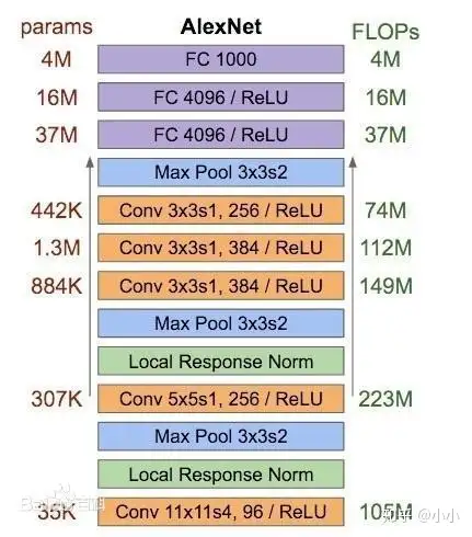
2012 年， AlexNet 横空出世。这个模型的名字来源于论⽂第一作者的姓名 Alex Krizhevsky。AlexNet 使⽤了 8 层卷积神经⽹络，并以很⼤的优势赢得了 ImageNet 2012 图像识别挑战赛冠军

Alexnet模型由5个卷积层和3个池化Pooling 层，其中还有3个全连接层构成。AlexNet 跟 LeNet 结构类似，但使⽤了更多的卷积层和更⼤的参数空间来拟合⼤规模数据集 ImageNet。它是浅层神经⽹络和深度神经⽹络的分界线

特点：

在每个卷机后面添加了Relu激活函数，解决了Sigmoid的梯度消失问题，使收敛更快。
使用随机丢弃技术（dropout）选择性地忽略训练中的单个神经元，避免模型的过拟合（也使用数据增强防止过拟合）
添加了归一化LRN（Local Response Normalization，局部响应归一化）层，使准确率更高。
重叠最大池化（overlapping max pooling），即池化范围 z 与步长 s 存在关系 z>s 避免平均池化（average pooling）的平均效应

AlexNet的网络架构

# input_size  (1, 1, 224, 224)
# output_size (1, 10)
class AlexNet(nn.Module):
    def __init__(self):
        super(AlexNet, self).__init__()
        self.conv = nn.Sequential(
            nn.Conv2d(1, 96, kernel_size=11, stride=4), nn.ReLU(),
            nn.BatchNorm2d(96),
            nn.MaxPool2d(kernel_size=3, stride=2),
            nn.Conv2d(96, 256, kernel_size=5, stride=1, padding=2), nn.ReLU(),
            nn.BatchNorm2d(256),
            nn.MaxPool2d(kernel_size=3, stride=2),
            nn.Conv2d(256, 384, kernel_size=3, stride=1, padding=1), nn.ReLU(),
            nn.Conv2d(384, 384, kernel_size=3, stride=1, padding=1), nn.ReLU(),
            nn.Conv2d(384, 256, kernel_size=3, stride=1, padding=1), nn.ReLU(),
            nn.MaxPool2d(kernel_size=3, stride=2),
        )
        self.linear = nn.Sequential(
            nn.Flatten(),
            nn.Linear(256 * 5 * 5, 4096), nn.ReLU(),
            nn.Dropout1d(p=0.5),
            nn.Linear(4096, 4096), nn.ReLU(),
            nn.Dropout1d(p=0.5),
            nn.Linear(4096, 10),
            nn.Softmax(dim=1),
        )
    
    def forward(self, X):
        X = self.conv(X)
        X = self.linear(X)
        return X

showNet(
    nn.Sequential(
            nn.Conv2d(1, 96, kernel_size=11, stride=4), nn.ReLU(),
            nn.BatchNorm2d(96),
            nn.MaxPool2d(kernel_size=3, stride=2),
            nn.Conv2d(96, 256, kernel_size=5, stride=1, padding=2), nn.ReLU(),
            nn.BatchNorm2d(256),
            nn.MaxPool2d(kernel_size=3, stride=2),
            nn.Conv2d(256, 384, kernel_size=3, stride=1, padding=1), nn.ReLU(),
            nn.Conv2d(384, 384, kernel_size=3, stride=1, padding=1), nn.ReLU(),
            nn.Conv2d(384, 256, kernel_size=3, stride=1, padding=1), nn.ReLU(),
            nn.MaxPool2d(kernel_size=3, stride=2),
            nn.Flatten(),
            nn.Linear(256 * 5 * 5, 4096), nn.ReLU(),
            nn.Dropout1d(p=0.5),
            nn.Linear(4096, 4096), nn.ReLU(),
            nn.Dropout1d(p=0.5),
            nn.Linear(4096, 10),
            nn.Softmax(dim=1),
    ), 
    (1, 1, 224, 224),
)

Conv2d output shape : torch.Size([1, 96, 54, 54])
ReLU output shape : torch.Size([1, 96, 54, 54])
BatchNorm2d output shape : torch.Size([1, 96, 54, 54])
MaxPool2d output shape : torch.Size([1, 96, 26, 26])
Conv2d output shape : torch.Size([1, 256, 26, 26])
ReLU output shape : torch.Size([1, 256, 26, 26])
BatchNorm2d output shape : torch.Size([1, 256, 26, 26])
MaxPool2d output shape : torch.Size([1, 256, 12, 12])
Conv2d output shape : torch.Size([1, 384, 12, 12])
ReLU output shape : torch.Size([1, 384, 12, 12])
Conv2d output shape : torch.Size([1, 384, 12, 12])
ReLU output shape : torch.Size([1, 384, 12, 12])
Conv2d output shape : torch.Size([1, 256, 12, 12])
ReLU output shape : torch.Size([1, 256, 12, 12])
MaxPool2d output shape : torch.Size([1, 256, 5, 5])
Flatten output shape : torch.Size([1, 6400])
Linear output shape : torch.Size([1, 4096])
ReLU output shape : torch.Size([1, 4096])
Dropout1d output shape : torch.Size([1, 4096])
Linear output shape : torch.Size([1, 4096])
ReLU output shape : torch.Size([1, 4096])
Dropout1d output shape : torch.Size([1, 4096])
Linear output shape : torch.Size([1, 10])
Softmax output shape : torch.Size([1, 10])
tensor([[0.1014, 0.0974, 0.0996, 0.1008, 0.1008, 0.1011, 0.0983, 0.1004, 0.1017, 0.0985]], grad_fn=)

VGG

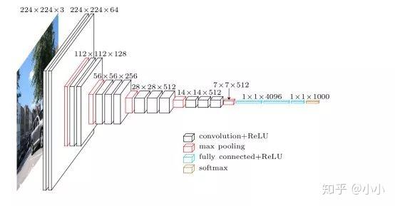
VGGNet 是由牛津大学视觉几何小组（Visual Geometry Group, VGG）提出的一种深层卷积网络结构，他们以 7.32% 的错误率赢得了 2014 年 ILSVRC 分类任务的亚军（冠军由 GoogLeNet 以 6.65% 的错误率夺得）和 25.32% 的错误率夺得定位任务（Localization）的第一名（GoogLeNet 错误率为 26.44%）。VGG可以看成是加深版本的AlexNet. 都是conv layer + FC layer

为了解决初始化（权重初始化）等问题，VGG采用的是一种Pre-training的方式，先训练浅层的的简单网络 VGG11，再复用 VGG11 的权重来初始化 VGG13，如此反复训练并初始化 VGG19，能够使训练时收敛的速度更快。整个网络都使用卷积核尺寸为 3×3 和最大池化尺寸 2×2

比较常用的VGG-16的16指的是conv+fc的总层数是16，是不包括max pool的层数！

3x3卷积的优点：

多个3×3的卷积层比一个大尺寸的filter有更少的参数，假设卷基层的输入和输出的特征图大小相同为C，那么三个3×3的卷积层参数个数3×（3×3×C×C）=27CC；一个7×7的卷积层参数为49CC；所以可以把三个3×3的filter看成是一个7×7filter的分解（中间层有非线性的分解）

VGG的网络架构

def vggBlock(conv_num, in_channels, out_channels):
    layers = []
    for _ in range(conv_num):
        layers.append(nn.Conv2d(in_channels, out_channels, kernel_size=3, stride=1, padding=1))
        layers.append(nn.ReLU())
        in_channels = out_channels
    layers.append(nn.MaxPool2d(kernel_size=2, stride=2))
    model = nn.Sequential(*layers)
    return model

def vgg(in_channels, conv_arch):
    conv_list = []
    for (conv_num, out_channels) in conv_arch:
        conv_list.append(vggBlock(conv_num, in_channels, out_channels))
        in_channels = out_channels
        
    return nn.Sequential(
        *conv_list,
        nn.Flatten(),
        nn.Linear(out_channels * 7 * 7, 4096), nn.ReLU(), nn.Dropout(p=0.5),
        nn.Linear(4096, 4096), nn.ReLU(), nn.Dropout(p=0.5),
        nn.Linear(4096, 10),
        nn.Softmax(dim=1),
    )

conv_arch = ((1, 64), (1, 128), (2, 256), (2, 512), (2, 512))
showNet(
    vgg(1, conv_arch),
    (1, 1, 224, 224),
)

Conv2d output shape : torch.Size([1, 96, 54, 54])
ReLU output shape : torch.Size([1, 96, 54, 54])
Conv2d output shape : torch.Size([1, 96, 54, 54])
ReLU output shape : torch.Size([1, 96, 54, 54])
Conv2d output shape : torch.Size([1, 96, 54, 54])
ReLU output shape : torch.Size([1, 96, 54, 54])
MaxPool2d output shape : torch.Size([1, 96, 26, 26])
Conv2d output shape : torch.Size([1, 256, 26, 26])
ReLU output shape : torch.Size([1, 256, 26, 26])
Conv2d output shape : torch.Size([1, 256, 26, 26])
ReLU output shape : torch.Size([1, 256, 26, 26])
Conv2d output shape : torch.Size([1, 256, 26, 26])
ReLU output shape : torch.Size([1, 256, 26, 26])
MaxPool2d output shape : torch.Size([1, 256, 12, 12])
Conv2d output shape : torch.Size([1, 384, 12, 12])
ReLU output shape : torch.Size([1, 384, 12, 12])
Conv2d output shape : torch.Size([1, 384, 12, 12])
ReLU output shape : torch.Size([1, 384, 12, 12])
Conv2d output shape : torch.Size([1, 384, 12, 12])
ReLU output shape : torch.Size([1, 384, 12, 12])
MaxPool2d output shape : torch.Size([1, 384, 5, 5])
Dropout output shape : torch.Size([1, 384, 5, 5])
Conv2d output shape : torch.Size([1, 10, 5, 5])
ReLU output shape : torch.Size([1, 10, 5, 5])
Conv2d output shape : torch.Size([1, 10, 5, 5])
ReLU output shape : torch.Size([1, 10, 5, 5])
Conv2d output shape : torch.Size([1, 10, 5, 5])
ReLU output shape : torch.Size([1, 10, 5, 5])
AdaptiveAvgPool2d output shape : torch.Size([1, 10, 1, 1])
Flatten output shape : torch.Size([1, 10])
Softmax output shape : torch.Size([1, 10])
tensor([[0.0893, 0.1014, 0.0876, 0.1105, 0.0876, 0.1088, 0.1234, 0.1086, 0.0896, 0.0930]], grad_fn=)

NiN

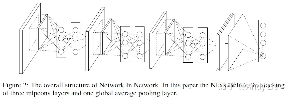
出自新加坡国立大学2014年的论文 Network In Network

该设计后来为 ResNet 和 Inception 等网络模型所借鉴

Improvement

先前CNN中简单的线性卷积层 [蓝框部分]被替换为了多层感知机（MLP，多层全连接层和非线性函数的组合） [绿框部分]：

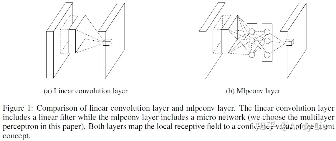
优点是：

提供了网络层间映射的一种新可能
增加了网络卷积层的非线性能力

先前CNN中的全连接层被替换为了全局池化层 (global average pooling)：

假设分类任务共有C个类别
先前CNN中最后一层为特征图层数共计N的全连接层，要映射到C个类别上；
改为全局池化层后，最后一层为特征图层数共计C的全局池化层，恰好对应分类任务的C个类别，这样一来，就会有更好的可解释性了

def ninBlock(in_channels, out_channels, kernel_size, stride, padding):
    model = nn.Sequential(
        nn.Conv2d(in_channels, out_channels, kernel_size, stride, padding), nn.ReLU(),
        nn.Conv2d(out_channels, out_channels, kernel_size=1), nn.ReLU(),
        nn.Conv2d(out_channels, out_channels, kernel_size=1), nn.ReLU(),
    )
    return model

showNet(
    nn.Sequential(
        ninBlock(1, 96, kernel_size=11, stride=4, padding=0),
        nn.MaxPool2d(3, stride=2),
        ninBlock(96, 256, kernel_size=5, stride=1, padding=2),
        nn.MaxPool2d(3, stride=2),
        ninBlock(256, 384, kernel_size=3, stride=1, padding=1),
        nn.MaxPool2d(3, stride=2),
        nn.Dropout(p=0.5),
        ninBlock(384, 10, kernel_size=3, stride=1, padding=1),
        nn.AdaptiveAvgPool2d((1, 1)),
        nn.Flatten(),
        nn.Softmax(dim=1),
    ),
    (1, 1, 224, 224),
)

Conv2d output shape : torch.Size([1, 96, 54, 54])
ReLU output shape : torch.Size([1, 96, 54, 54])
Conv2d output shape : torch.Size([1, 96, 54, 54])
ReLU output shape : torch.Size([1, 96, 54, 54])
Conv2d output shape : torch.Size([1, 96, 54, 54])
ReLU output shape : torch.Size([1, 96, 54, 54])
MaxPool2d output shape : torch.Size([1, 96, 26, 26])
Conv2d output shape : torch.Size([1, 256, 26, 26])
ReLU output shape : torch.Size([1, 256, 26, 26])
Conv2d output shape : torch.Size([1, 256, 26, 26])
ReLU output shape : torch.Size([1, 256, 26, 26])
Conv2d output shape : torch.Size([1, 256, 26, 26])
ReLU output shape : torch.Size([1, 256, 26, 26])
MaxPool2d output shape : torch.Size([1, 256, 12, 12])
Conv2d output shape : torch.Size([1, 384, 12, 12])
ReLU output shape : torch.Size([1, 384, 12, 12])
Conv2d output shape : torch.Size([1, 384, 12, 12])
ReLU output shape : torch.Size([1, 384, 12, 12])
Conv2d output shape : torch.Size([1, 384, 12, 12])
ReLU output shape : torch.Size([1, 384, 12, 12])
MaxPool2d output shape : torch.Size([1, 384, 5, 5])
Dropout output shape : torch.Size([1, 384, 5, 5])
Conv2d output shape : torch.Size([1, 10, 5, 5])
ReLU output shape : torch.Size([1, 10, 5, 5])
Conv2d output shape : torch.Size([1, 10, 5, 5])
ReLU output shape : torch.Size([1, 10, 5, 5])
Conv2d output shape : torch.Size([1, 10, 5, 5])
ReLU output shape : torch.Size([1, 10, 5, 5])
AdaptiveAvgPool2d output shape : torch.Size([1, 10, 1, 1])
Flatten output shape : torch.Size([1, 10])
Softmax output shape : torch.Size([1, 10])
tensor([[0.0893, 0.1014, 0.0876, 0.1105, 0.0876, 0.1088, 0.1234, 0.1086, 0.0896, 0.0930]], grad_fn=)

GoogLeNet

GoogLeNet是google推出的基于Inception模块的深度神经网络模型，在2014年的ImageNet竞赛中夺得了冠军，在随后的两年中一直在改进，形成了Inception V2、Inception V3、Inception V4等版本。我们会用一系列文章，分别对这些模型做介绍。本篇文章先介绍最早版本的GoogLeNet

1. 为什么要提出Inception

一般来说，提升网络性能最直接的办法就是增加网络深度和宽度，但一味地增加，会带来诸多问题：

参数太多，如果训练数据集有限，很容易产生过拟合；
网络越大、参数越多，计算复杂度越大，难以应用；
网络越深，容易出现梯度弥散问题（梯度越往后穿越容易消失），难以优化模型。

我们希望在增加网络深度和宽度的同时减少参数，为了减少参数，自然就想到将全连接变成稀疏连接。但是在实现上，全连接变成稀疏连接后实际计算量并不会有质的提升，因为大部分硬件是针对密集矩阵计算优化的，稀疏矩阵虽然数据量少，但是计算所消耗的时间却很难减少。在这种需求和形势下，Google研究人员提出了Inception的方法。

2. 什么是Inception

Inception就是把多个卷积或池化操作，放在一起组装成一个网络模块，设计神经网络时以模块为单位去组装整个网络结构。模块如下图所示

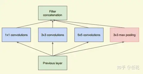
在未使用这种方式的网络里，我们一层往往只使用一种操作，比如卷积或者池化，而且卷积操作的卷积核尺寸也是固定大小的。但是，在实际情况下，在不同尺度的图片里，需要不同大小的卷积核，这样才能使性能最好，或者或，对于同一张图片，不同尺寸的卷积核的表现效果是不一样的，因为他们的感受野不同。所以，我们希望让网络自己去选择，Inception便能够满足这样的需求，一个Inception模块中并列提供多种卷积核的操作，网络在训练的过程中通过调节参数自己去选择使用，同时，由于网络中都需要池化操作，所以此处也把池化层并列加入网络中。

3. 实际中需要什么样的Inception

我们在上面提供了一种Inception的结构，但是这个结构存在很多问题，是不能够直接使用的。首要问题就是参数太多，导致特征图厚度太大。为了解决这个问题，作者在其中加入了1X1的卷积核，改进后的Inception结构如下图

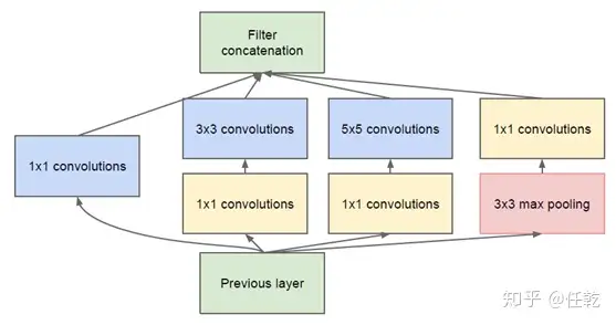
这样做有两个好处，首先是大大减少了参数量，其次，增加的1X1卷积后面也会跟着有非线性激励，这样同时也能够提升网络的表达能力

GoogLeNet采用了模块化的结构（Inception结构），方便增添和修改；
网络最后采用了average pooling（平均池化）来代替全连接层，该想法来自NIN（Network in Network），事实证明这样可以将准确率提高0.6%。
虽然移除了全连接，但是网络中依然使用了Dropout ;

class Inception(nn.Module):
    def __init__(self, in_channels, c1, c2, c3, c4, **kwargs):
        super(Inception, self).__init__(**kwargs)
        self.p1 = nn.Sequential(
            nn.Conv2d(in_channels, c1, kernel_size=1),
            nn.ReLU(),
        )
        self.p2 = nn.Sequential(
            nn.Conv2d(in_channels, c2[0], kernel_size=1),
            nn.Conv2d(c2[0], c2[1], kernel_size=3, padding=1),
            nn.ReLU(),
        )
        self.p3 = nn.Sequential(
            nn.Conv2d(in_channels, c3[0], kernel_size=1),
            nn.Conv2d(c3[0], c3[1], kernel_size=5, padding=2),
            nn.ReLU(),
        )
        self.p4 = nn.Sequential(
            nn.MaxPool2d(kernel_size=3, stride=1, padding=1),
            nn.Conv2d(in_channels, c4, kernel_size=1),
            nn.ReLU(),
        )
        
    def forward(self, inputs):
        p1 = self.p1(inputs)
        p2 = self.p2(inputs)
        p3 = self.p3(inputs)
        p4 = self.p4(inputs)
        inputs = torch.cat((p1, p2, p3, p4), dim=1)
        return inputs

showNet(
    nn.Sequential(
        nn.Sequential(
            nn.Conv2d(1, 64, kernel_size=7, stride=2, padding=3),
            nn.ReLU(),
            nn.MaxPool2d(kernel_size=3, stride=2, padding=1),
        ),
        nn.Sequential(
            nn.Conv2d(64, 64, kernel_size=1),
            nn.ReLU(),
            nn.Conv2d(64, 192, kernel_size=3, padding=1),
            nn.ReLU(),
            nn.MaxPool2d(kernel_size=3, stride=2, padding=1),
        ),
        nn.Sequential(
            Inception(192, 64, (96, 128), (16, 32), 32),
            Inception(256, 128, (128, 192), (32, 96), 64),
            nn.MaxPool2d(kernel_size=3, stride=2, padding=1),
        ),
        nn.Sequential(
            Inception(480, 192, (96, 208), (16, 48), 64),
            Inception(512, 160, (112, 224), (24, 64), 64),
            Inception(512, 128, (128, 256), (24, 64), 64),
            Inception(512, 112, (144, 288), (32, 64), 64),
            Inception(528, 256, (160, 320), (32, 128), 128),
            nn.MaxPool2d(kernel_size=3, stride=2, padding=1),
        ),
        nn.Sequential(
            Inception(832, 256, (160, 320), (32, 128), 128),
            Inception(832, 384, (192, 384), (48, 128), 128),
            nn.AdaptiveAvgPool2d((1, 1)),
            nn.Flatten(),
            nn.Linear(1024, 10),
            nn.Softmax(dim=1),
        ),
    ),
    (1, 1, 224, 224),
)

Conv2d output shape : torch.Size([1, 64, 112, 112])
ReLU output shape : torch.Size([1, 64, 112, 112])
MaxPool2d output shape : torch.Size([1, 64, 56, 56])
Conv2d output shape : torch.Size([1, 64, 56, 56])
ReLU output shape : torch.Size([1, 64, 56, 56])
Conv2d output shape : torch.Size([1, 192, 56, 56])
ReLU output shape : torch.Size([1, 192, 56, 56])
MaxPool2d output shape : torch.Size([1, 192, 28, 28])
Inception output shape : torch.Size([1, 256, 28, 28])
Inception output shape : torch.Size([1, 480, 28, 28])
MaxPool2d output shape : torch.Size([1, 480, 14, 14])
Inception output shape : torch.Size([1, 512, 14, 14])
Inception output shape : torch.Size([1, 512, 14, 14])
Inception output shape : torch.Size([1, 512, 14, 14])
Inception output shape : torch.Size([1, 528, 14, 14])
Inception output shape : torch.Size([1, 832, 14, 14])
MaxPool2d output shape : torch.Size([1, 832, 7, 7])
Inception output shape : torch.Size([1, 832, 7, 7])
Inception output shape : torch.Size([1, 1024, 7, 7])
AdaptiveAvgPool2d output shape : torch.Size([1, 1024, 1, 1])
Flatten output shape : torch.Size([1, 1024])
Linear output shape : torch.Size([1, 10])
Softmax output shape : torch.Size([1, 10])
tensor([[0.1017, 0.0981, 0.0969, 0.1013, 0.1027, 0.1005, 0.0995, 0.1007, 0.0990, 0.0995]], grad_fn=)

DenseNet

相比ResNet，DenseNet提出了一个更激进的密集连接机制：即互相连接所有的层，具体来说就是每个层都会接受其前面所有层作为其额外的输入。图1为ResNet网络的连接机制，作为对比，图2为DenseNet的密集连接机制。可以看到，ResNet是每个层与前面的某层（一般是2~3层）短路连接在一起，连接方式是通过元素级相加。而在DenseNet中，每个层都会与前面所有层在channel维度上连接（concat）在一起（这里各个层的特征图大小是相同的，后面会有说明），并作为下一层的输入。对于一个L层的网络，DenseNet共包含L(L + 1) / 2个连接，相比ResNet，这是一种密集连接。而且DenseNet是直接concat来自不同层的特征图，这可以实现特征重用，提升效率，这一特点是DenseNet与ResNet最主要的区别

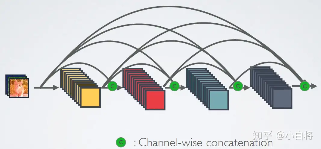
CNN网络一般要经过Pooling或者stride>1的Conv来降低特征图的大小，而DenseNet的密集连接方式需要特征图大小保持一致。为了解决这个问题，DenseNet网络中使用DenseBlock+Transition的结构，其中DenseBlock是包含很多层的模块，每个层的特征图大小相同，层与层之间采用密集连接方式。而Transition模块是连接两个相邻的DenseBlock，并且通过Pooling使特征图大小降低。图4给出了DenseNet的网路结构，它共包含4个DenseBlock，各个DenseBlock之间通过Transition连接在一起

DenseNet的优势主要体现在以下几个方面：

由于密集连接方式，DenseNet提升了梯度的反向传播，使得网络更容易训练。由于每层可以直达最后的误差信号，实现了隐式的“deep supervision”；
参数更小且计算更高效，这有点违反直觉，由于DenseNet是通过concat特征来实现短路连接，实现了特征重用，并且采用较小的growth rate，每个层所独有的特征图是比较小的；
由于特征复用，最后的分类器使用了低级特征。

def conv_block(input_channels, num_channels):
    return nn.Sequential(
        nn.BatchNorm2d(input_channels), nn.ReLU(),
        nn.Conv2d(input_channels, num_channels, kernel_size=3, padding=1),
    )

class DenseBlock(nn.Module):
    def __init__(self, num_conv, input_channels, num_channels):
        super(DenseBlock, self).__init__()
        layer = []
        for i in range(num_conv):
            layer.append(conv_block(num_channels * i + input_channels, num_channels))
        self.net = nn.Sequential(*layer)
        
    def forward(self, X):
        for blk in self.net:
            Y = blk(X)
            X = torch.cat((X, Y), dim=1)
        return X

def transition_block(input_channels, num_channels):
    return nn.Sequential(
        nn.BatchNorm2d(input_channels), nn.ReLU(),
        nn.Conv2d(input_channels, num_channels, kernel_size=1),
        nn.AvgPool2d(kernel_size=2, stride=2),
    )

def DenseNet(num_channels, growth_rate, num_convs):
    b1 = nn.Sequential(
        nn.Conv2d(1, 64, kernel_size=7, stride=2, padding=3),
        nn.BatchNorm2d(64), nn.ReLU(),
        nn.MaxPool2d(kernel_size=3, stride=2, padding=1),
    )
    blk = []
    for i, num_conv in enumerate(num_convs):
        blk.append(DenseBlock(num_conv, num_channels, growth_rate))
        num_channels += num_conv * growth_rate
        if i != len(num_convs) - 1:
            blk.append(transition_block(num_channels, num_channels // 2))
            num_channels = num_channels // 2
    b2 = nn.Sequential(
        nn.BatchNorm2d(num_channels), nn.ReLU(),
        nn.AdaptiveAvgPool2d((1, 1)),
        nn.Flatten(),
        nn.Linear(num_channels, 10),
        nn.Softmax(dim=1),
    )
    return nn.Sequential(
        b1,
        *blk,
        b2,
    )

showNet(
    DenseNet(
        64,
        32,
        [4, 4, 4, 4],
    ),
    (1, 1, 224, 224),
)

Conv2d output shape : torch.Size([1, 64, 112, 112])
BatchNorm2d output shape : torch.Size([1, 64, 112, 112])
ReLU output shape : torch.Size([1, 64, 112, 112])
MaxPool2d output shape : torch.Size([1, 64, 56, 56])
DenseBlock output shape : torch.Size([1, 192, 56, 56])
BatchNorm2d output shape : torch.Size([1, 192, 56, 56])
ReLU output shape : torch.Size([1, 192, 56, 56])
Conv2d output shape : torch.Size([1, 96, 56, 56])
AvgPool2d output shape : torch.Size([1, 96, 28, 28])
DenseBlock output shape : torch.Size([1, 224, 28, 28])
BatchNorm2d output shape : torch.Size([1, 224, 28, 28])
ReLU output shape : torch.Size([1, 224, 28, 28])
Conv2d output shape : torch.Size([1, 112, 28, 28])
AvgPool2d output shape : torch.Size([1, 112, 14, 14])
DenseBlock output shape : torch.Size([1, 240, 14, 14])
BatchNorm2d output shape : torch.Size([1, 240, 14, 14])
ReLU output shape : torch.Size([1, 240, 14, 14])
Conv2d output shape : torch.Size([1, 120, 14, 14])
AvgPool2d output shape : torch.Size([1, 120, 7, 7])
DenseBlock output shape : torch.Size([1, 248, 7, 7])
BatchNorm2d output shape : torch.Size([1, 248, 7, 7])
ReLU output shape : torch.Size([1, 248, 7, 7])
AdaptiveAvgPool2d output shape : torch.Size([1, 248, 1, 1])
Flatten output shape : torch.Size([1, 248])
Linear output shape : torch.Size([1, 10])
Softmax output shape : torch.Size([1, 10])
tensor([[0.1015, 0.0667, 0.0933, 0.1145, 0.1166, 0.0881, 0.0913, 0.1304, 0.0918, 0.1058]], grad_fn=)

总结

LeNet

卷积神经网络概念的提出
分为卷积层和全连接层
没用到 Dropout 和 BatchNormal 等正则化技术

AlexNet

深度卷积神经网络的第一次尝试
分为卷积层和全连接层
卷积层使用了暂退法，Dropout
全连接层使用了批量正则化 BatchNormal

VGG

可以看作是模块化了的 AlexNet
网络模块化，可便捷加深或预训练
不断地使用卷积 + 池化，最后全连接
可使用相关正则化技术

NiN

先不断地卷积 + 多层感知机连接(即一维卷积核)
然后不断地池化，最后池化至 (1, 1)
最终每个通道的值对应一个分类的预测值

GoogleNet

可模块化
大大减少了网络参数，优化了显存消耗
每层可实现多种操作，扩大了感受野
不使用全连接，可 Dropout

ResNet

每层采用恒等变换，扩大了网络的可变性
为每层网络的训练提供快捷通道，极大地消除了深层网络的训练问题
极大地启发了往后深度网络的架构思路

DenseNet

每个层都会接受其前面所有层作为其额外的输入
实现特征复用，简单特征居多
特征计算小，网络训练高效
不断地扩大特征并池化，使网络在一边增长的同时一边缩减